89  Ensemble Methods in ML

89.1 Introduction

‘Ensemble methods’ in ML leverage the power of multiple learning algorithms to achieve better predictive performance than could be obtained from any of the individual learning models alone.

This approach is based on the principle that a group of “weak learners” can come together to form a “strong learner,” and improve the robustness and accuracy of predictions.

The core idea behind ensemble methods is to combine the predictions of several models (e.g., classifiers or regressors) to correct errors made by individual models. It’s an example of the phrase ‘two minds are better than one’.

There are two main types of ensemble methods: ‘boosting’ and ‘bagging’.

• Boosting: This method builds a series of models in a sequential manner, where each subsequent model attempts to correct the errors of its predecessor.

• Bagging (Bootstrap Aggregating): Unlike boosting, bagging trains each model in the ensemble independently from the others using a randomly drawn subset of the training set (with replacement).

89.2 Bagging

Introduction

‘Bagging’, or ‘Bootstrap Aggregating’, is an ensemble learning technique used to improve the stability and accuracy of machine learning algorithms, particularly decision trees.

By creating multiple versions of a predictor model and training each one on a random subset of the training data, bagging reduces the variance of the prediction error and helps prevent overfitting.

We learned about random forests earlier in the module, which are a great example of this technique.

In bagging, each model in the ensemble is built from a bootstrap sample. A ‘bootstrap sample’ is a randomly drawn sample of the training data, selected with replacement.

This results in different subsets of the data being used for training different models, introducing diversity among the models in the ensemble.

The final output is typically obtained by averaging the predictions (for regression problems) or by majority voting (for classification problems).

Bagging is particularly effective for algorithms with high variance and low bias, as it works by averaging out the variance without significantly increasing bias. By leveraging the strength of multiple learners, bagging can significantly improve model accuracy and robustness across various domains and applications in machine learning.

You can read more here.

Example

We used the iris dataset earlier in the module. Now, we’ll use it to demonstrate the random forest approach to building a classification model.

As you know, after we train our model, we can examine the confusion matrix to see how well our model it performs.

Code

library(randomForest)

randomForest 4.7-1.1

Type rfNews() to see new features/changes/bug fixes.

Code

# Using the iris dataset
data(iris)
x <- iris[, -5]  # Feature variables (all columns except the species)
y <- iris[, 5]   # Target variable (species column)

# Train the random forest model
set.seed(42)  # For reproducibility
rf_model <- randomForest(x = x, y = y, ntree = 100)

# Print the model summary
print(rf_model)

Call:
 randomForest(x = x, y = y, ntree = 100) 
               Type of random forest: classification
                     Number of trees: 100
No. of variables tried at each split: 2

        OOB estimate of  error rate: 4%
Confusion matrix:
           setosa versicolor virginica class.error
setosa         50          0         0        0.00
versicolor      0         47         3        0.06
virginica       0          3        47        0.06

Code

# Plot variable importance
importance <- importance(rf_model)
varImpPlot(rf_model)

The ntree = 100 argument specifies that we want our forest to consist of 100 trees. After training, the model summary printed gives an overview of the model’s performance, including the confusion matrix and the percentage of correctly classified instances.

89.3 Boosting

Introduction

‘Boosting’ is another ensemble technique that aims to create a strong classifier from a number of weak classifiers.

Unlike bagging, this method sequentially builds the ensemble by training each new model to emphasise the training instances that previous models misclassified. In boosting, the models are built sequentially by adjusting the weights of incorrectly classified instances so that subsequent models focus more on difficult cases.

Each model in the sequence is trained using a weighted form of the data. Initially, all data points have equal weights, but as training progresses, the algorithm increases the weights of the instances that are hard to predict and decreases the weights for those that are easy to predict. This iterative approach allows the ensemble to focus on the more challenging aspects of the training data.

One of the key features of boosting is that it combines multiple weak or moderate learners to create a strong learner. Each weak learner contributes its strengths, compensating for the weaknesses of others, which results in improved accuracy and performance of the ensemble.

Popular boosting algorithms include AdaBoost (Adaptive Boosting) and Gradient Boosting.

• AdaBoost adjusts the weights of misclassified data points after each iteration and combines the weak learners into a weighted sum that represents the final output of the boosted classifier.

• Gradient Boosting builds models sequentially, with each new model being trained to correct the errors made by the previous ones, using a gradient descent algorithm to minimise the loss when adding the latest model.

Confused?

Imagine you’re playing a video game where you need to get past several levels, and each level is a bit harder than the last one. Now, suppose you’re not alone – you’ve got a group of friends helping you out. Each friend takes a turn to play a level. If they get through it, great! But if they don’t, the next friend pays extra attention to where things went wrong and tries to do better on that part.

In machine learning, “boosting” is like this team effort to win the game. Instead of friends, you have a group of helpers called “models” that try to predict something (like whether a photo shows an orange or an apple).

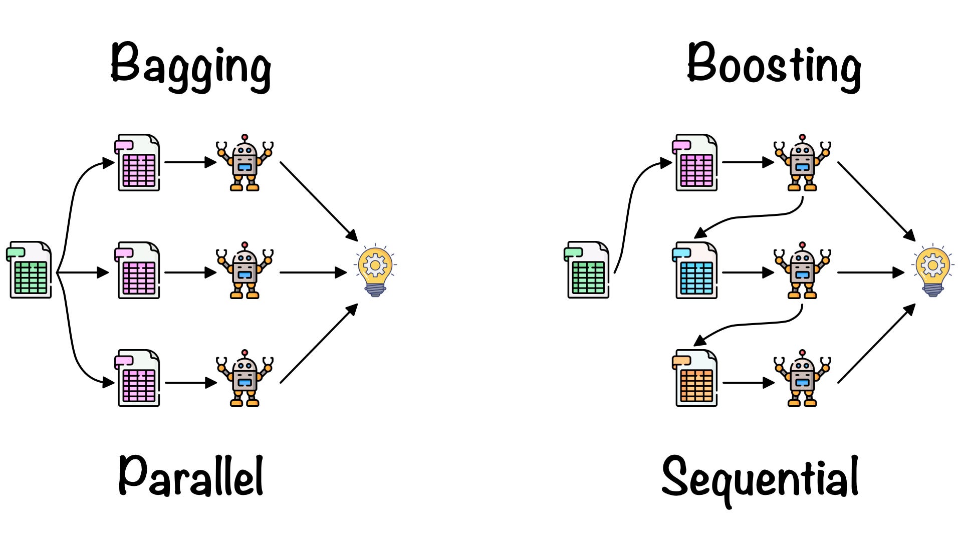
The first model makes its best guess, but it probably doesn’t get everything right. So, the next model watches and ‘learns’ from the mistakes of the first model, trying specifically to get those wrong predictions right, giving more focus to the harder parts. This process goes on with several models, each one learning from the errors of the one before it, and paying more attention to the things that are harder to predict.

In the end, all these models come together, combining their strengths, and make a final, super-smart guess. Just like how you and your friends would combine your gaming skills to win the video game, these models join forces to make a really good prediction.

Example

Here’s an example of a gradient boosted model applied to the iris dataset. The GBM creates a ‘perfect’ model, which predicts the dichotomous outcome 100% correctly.

Code

library(gbm)

# Load the iris dataset
data(iris)

# Convert the Species to a binary classification task
# create a binary variable indicating whether the species is Setosa or not
iris$IsSetosa <- ifelse(iris$Species == "setosa", 1, 0)

# Split the dataset into training and testing sets
set.seed(42)  # Ensure reproducibility
index <- sample(1:nrow(iris), 0.7 * nrow(iris))  # 70% for training
train_data <- iris[index, ]
test_data <- iris[-index, ]

# Train the GBM model
# predict 'IsSetosa' using the other features
gbm_model <- gbm(IsSetosa ~ ., data = train_data, distribution = "bernoulli", 
                 n.trees = 100, interaction.depth = 1, shrinkage = 0.01, 
                 n.minobsinnode = 10, verbose = FALSE)

# Model summary
summary(gbm_model)

                      var  rel.inf
Petal.Length Petal.Length 57.97045
Species           Species 42.02955
Sepal.Length Sepal.Length  0.00000
Sepal.Width   Sepal.Width  0.00000
Petal.Width   Petal.Width  0.00000

Code

# Prediction and evaluation
# Note: We use the test data without the 'IsSetosa' column for prediction
predicted_probs <- predict(gbm_model, newdata = test_data, n.trees = 100, type = "response")
predicted_classes <- ifelse(predicted_probs > 0.5, 1, 0)

# Calculate the accuracy
accuracy <- mean(predicted_classes == test_data$IsSetosa)
cat("Accuracy:", accuracy, "\n")

Accuracy: 1